Monte Carlo Analysis in AmiBroker

This post will cover in detail two different ways of doing Monte Carlo analysis and the code needed to it in AmiBroker. A reader recently sent me this article, Monte Carlo Analysis For Trading Systems. The article covers three methods of Monte Carlo analysis. One of which I had never thought about and I had to slap my head on how simple it was.

What is Monte Carlo analysis?

The general idea behind Monte Carlo analysis is to add randomness to one’s strategy and see how it performs. You do this several hundred to several thousand times and one can compute the average, standard deviation of all the runs for CAR, Drawdowns, and other portfolio statistics. The idea being does the system behave well when some randomness is added? We will explore in depth two ways of doing Monte Carlo analysis in AmiBroker.

The Mean Reversion Strategy

To run on Monte Carlo analysis on, we will use a simple mean reversion strategy.

Test from 1/1/2004 to 6/30/2014. Maximum of 10 open positions at one time.

Setup Rules

• Stock is a member of the Russell 3000
• The 21 day moving average of Close*Volume is greater than $5,000,000
• Close is greater than $1
• Two period RSI is less than 7.5
• Has closed down 4 days in a row
• Close is above the 200 day moving average
• The 100 day Historical Volatility is greater than 40

Buy Rules

• Rank stocks from Highest 100 day Historical Volatility to lowest
• Buy the top 10 stocks
• Buy on the next open

Sell Rules

• Two period RSI closes above 30
• Sell on the next open

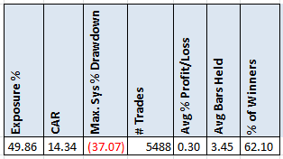
Base Results

Not a strategy that most people would trade but this gives us something to work with.

Randomizing trade order (Method 0)

This method uses all the trades that the strategy took but then randomly selects the order they happened in. This method is best employed when trading a single symbol. The issue with doing this when trading a portfolio of symbols is that trades are often correlated together. For example a mean reversion strategy during a market has a sell off. Typically most of trades are losers during this time. Monte Carlo analysis does not account for this behavior. Doing this type of testing in AmiBroker is not straightforward.

Adding noise to the rules (Method 1)

For method 2, one varies the rule values by a small percentage. Take the RSI(2) < 7.5 rule. What we do is vary 7.5 by a little. Instead of 7.5, we use 6.82 or 9.84. One would set the code to vary the rule value by a percentage. Using this method, the strategy generates a different set of trades each time. One advantage of this method over the previous one is that if the strategy did well because of a handful of trades, this analysis would potential discover that.

The randomness to the rule values can be added three ways. Each case adds more randomness. We will use the RSI(2) < 7.5 as an example below.

1. The random value for RSI would be the same for every stock on every day.
2. The random value for RSI would be different for every stock but the same on every day
3. The random value for RSI would be different for every stock and every day.

AmiBroker Code to add randomness for item 3 above follows, which is also the easiest to do in AmiBroker.

// returns a random array between 1*(1-percent) and 1*(1+percent)
// For example a percent=10 returns random numbers between .9 and 1.1

function RandPercent(percent)
{
     perc = percent/100;
     rand = 1+(perc - Random() * (perc*2));

     return rand;

}

minRSI = 7.5*RandPercent(20);
minHV = 40*RandPercent(10);
exitRSI = 30*RandPercent(5);

The above code would set a 20% range for the RSI(2) < 7.5 rule. The RSI values would be between 6 and 9. The range is up to the user. Here, 20% seemed to give a good range of values. For the historical volatility we vary the value by 10%, which is range from 36 to 40. For the exit RSI we by 5%, a little small but I wanted to show different values. The range would be from 28.5 to 31.5.

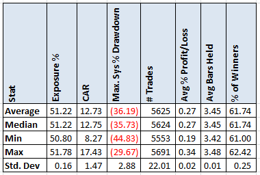
Method 1 Results

Note that the average and median values for the CAR of 12.7 are below the base results of 14.3. One would like to see this much closer together. The Monte Carlo simulation tells us to expect about a 11% less return. Even the worst run for CAR and MDD would be within what I would consider acceptable range. Not that I could trade a strategy with a 45% drawdown which few people can.

Adding noise to stock data (Method 2)

This is the method that I had not thought about before and had a head slapping moment on how simple it is. We apply the noise to the stock data values. For this example, we will apply the noise to the closing prices. Closing prices are randomly adjusted by a small percentage. The closing price need only vary by a little bit to have an impact in the results. Using a value of .25%, means that the closing price each day can be between .25% lower to .25% higher. A quarter percent is very little but for rules like RSI2 and closing down days it can have a significant impact.

This method also generates a different trade list every time. Since we are not applying the randomness to the Opening price, the return of a stock is not affected.

AmiBroker Code to add randomness for this method.

// returns a random array between 1*(1-percent) and 1*(1+percent)
// For example a percent=10 returns random numbers between .9 and 1.1

function RandPercent(percent)
{
     perc = percent/100;
     rand = 1+(perc - Random() * (perc*2));
     return rand;
}

Close = Close * RandPercent(.25); // varying the close price by .25%

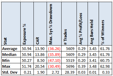
Method 2 Results

As one can see, these numbers differ from Method 1. The CAR of 13.9 is much closer to the base CAR of 14.3. The standard deviation for CAR is much higher but that is because one has higher return simulations.

Spreadsheet & Code

Fill the form in below for the spreadsheet of the results, yearly breakdown and the AmiBroker code used to generate them. The code assumes that Norgate Data is your data provider and that you have the Platinum level.

Final Thoughts

Which method should one use? It is up to you and which method makes the more sense to you. Both methods give similar results, which is good to see. Method 2 is my preference because it is easier to implement and I like that it is changing the closing price. If my rules used the low (or open or high) price, then I would add randomness to the low price.

I do not always run Monte Carlo analysis on my strategies as formally defined. I use a method very similar to “adding noise to the rules.” But now that I have purchased a new blazingly fast computer, I will do more Monte Carlos analysis in the future using method 2.

Backtesting platform used: AmiBroker. Data provider:Norgate Data (referral link)

Good quant trading,