Multiple Time Frames for Scoring ETF Rotational Strategies

Today we have a guest post from David Weilmuenster who I worked with while at Connors Research.

A widely applied technique for scoring assets in rotational systems is to rank those assets by their price momentum, or return, over a given historical window and to rotate into the assets with higher momentum. This approach seeks to capitalize on the well-demonstrated tendency for price momentum to persist. But, it begs some questions:

1. “What is an appropriate historical period for measuring price momentum?” Clearly, the momentum of a given asset can rank quite differently compared to the tradable universe over 1 month, 3 months, or 6 months.
2. “Is one historical period sufficient?” If relative momentum can vary widely depending on the historical window, would it be better to consider multiple slices of history?
3. Is higher momentum always preferable to lower momentum, especially if the system rules filter the tradable universe before scoring the ETFs for rotation?

Let’s see what we can learn about these questions from a straightforward system that rotates monthly among ETFs that represent the following 4 categories of worldwide assets:

• Equities (pre-dominantly stocks of operating companies)
• Fixed Income (bonds, preferred stocks, etc.)
• Commodities (broad markets, precious metals, energy)
• Real Estate

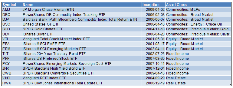
The universe we will trade is:

And, the trading system is:

• Test Dates: 2007-01-01 through 2014-12-31
• Rotate Monthly, taking signals from last trading day of the month, and entering/exiting on the Open of the first trading day of the subsequent month.
• 3 maximum positions, with equal size, i.e., 33.3% of Equity. (Results for 2 & 4 position portfolios are shown in a spreadsheet that you can request below).

• Filtering (each of these is tested separately):
  • No filtering.
  • ETFs are candidates for the next rotation only when trading at prices above 90% of their weekly closes for the past year.

• Rotational Score: A weighted average of the ranks of 1 month, 3 month, and 6 month returns.

The highest returns are ranked as 1 for each rotation, and lower returns have progressively higher ranks, so a negative weight favors higher returns. If only one of the weights is non-zero, then we are scoring only on the return from the related historical period.

For example, weights of -20, -40, & 40 favor higher returns for 1 and 3 months, and lower returns for 6 months. Weights of 0, -100, & 0, favor ETFs with higher returns for the previous 3 months, regardless of 1 and 6 month momentum.

We aren’t attempting here to design the best possible portfolio, but to generate a credible system that allows us to analyze the effects of different approaches to rotation scoring.

Here’s the performance of the variations that use no filtering and only a single timeframe to score assets for rotation (again, all variations are available in a spreadsheet that you can request below.) Remember that negative scores favor higher returns. “Adjusted CAR (Compound Annual Return)” is calculated by substituting the median 12 month rolling return for the highest 12 month return. Adjusted CAR helps us to avoid a bias toward variations with high CAR that results mostly from a single, exceptionally high 12 month return:

Even though the results aren’t attractive due to the high drawdowns, performance definitely improves when favoring higher returns (negative weight) for a given historical timeframe. The 1 month historical period is generally the best option in this case.

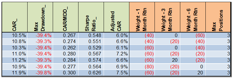
Next are the “Top Performers” when using no filtering and employing either a single timeframe, or multiple timeframes, for rotation scoring. “Top Performers” are in the Top 10 for every one of the following 4 metrics:

• CAR
• Adjusted CAR
• CAR / Maximum Daily Drawdown (CAR/MDD)
• Sharpe Ratio

Note that all of the top performers incorporate multiple timeframes into the rotation score. And, some of the variations emphasize lower price momentum (positive weights) for certain timeframes.

The filtering method described above can reduce the drawdowns. Here are the variations that use filtering and only a single timeframe for scoring:

Notice we now have an “anti-momentum” effect. The variation scored only by lowest 3 month momentum has the 2nd highest CAR (10.7%, practically identical to the highest CAR), and the highest CAR/MDD, Sharpe Ratio, and Adjusted CAR. So higher momentum isn’t always the most effective choice depending on how one filters the universe of assets and one’s preferred performance metrics.

Next are the top performers when using filtering and either single or multiple timeframes for scoring.

Now (for my money) the best weighting yields a 12.8% CAR by favoring higher 1 and 6 month returns, and lower 3 month returns. You might prefer another variation, but all of the top performers incorporate multiple timeframes in the scoring.

So, how do we answer the questions at the start of this post:

• “What is an appropriate historical period for measuring price momentum?”

For this system, the most recent month’s momentum does best when using only one historical timeframe for ranking. But, we had to evaluate test results to learn that. No theory could have predicted that 1 month was better than 3 months, or 6 months. Testing different possibilities is essential.

• “Is one historical period sufficient?”

For this system, it’s generally better to incorporate more than one historical timeframe in the ranking algorithm. This doesn’t prove that multiple timeframes are better for all systems, but experience suggests that it usually pays.

• Is higher momentum always preferable to lower momentum, especially if the system rules filter the tradable universe before scoring the ETFs for rotation?

Filtering in this system clearly has a substantial impact on whether to favor higher or lower momentum, and in what timeframe. Again, this isn’t proof for all systems, but a good tip to remember when creating your own systems.

How does this example compare to your experience in creating rotational systems?

Backtesting platform used: AmiBroker. Data provider:Norgate Data (referral link)

David Weilmuenster

Fill in for free spreadsheet:

Contains yearly breakdown, different weightings and more.