- in Mean Reversion , Research , Stocks by Cesar Alvarez
Optimization Mean Reversion
Often one runs a optimization of a testing idea, then using some set metrics from these results, one picks a variation to trade. What often comes as a surprise to people, and myself the first time I saw this, is that your optimization runs are often mean reverting. What do I mean by this?
For example, you have a 100 run optimization from 2000 to 2012. Now you sort by your metric, say Compound Annual Return. Now do the same optimization from 2013 to 2015. You will notice that your top runs from the first period moving toward the middle of the second period. And your bottom runs of the first period moving to the middle in the second period. Let us look at some tests and data.
The Test
Period 1 from 1/1/2000 to 12/31/2012. Period 2 from 1/1/2013 to 12/31/2015.
Buy Rules
- Stock is member of S&P500 index
- Close is under 5 day moving average for (3,4,5,6,7) days
- Stock closes in the bottom (10, 20, 30, 40, 50)% of the daily range. This is known as Closing Range or Internal Bar Strength
- Close is above the (50,100,150,200) day moving average
- Close of SPX is above the 200 day moving average of SPX
- Enter on next open
Sell Rules
- Close is above 5 day moving average for (1,2,3) days
This is a simple mean reversion strategy. I picked the number of parameters to optimize on so I would get enough variations to give my deciles enough samples.
Analysis
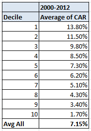
Given the above rules, this produces 2520 variations. I ran an optimization over the first time period. I then sorted the data by Compound Annual Return and divided it into deciles.

The CAR of the SPY during this period is 1.70%. An interesting thing is wide the range is. Part of this is explained because some of the variations produce very low exposure.
Comparing to 2013 to 2015
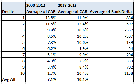
Next, I ran the same optimization over the second time period. For each decile of the first time period, I looked at each variation to see what the rank was in the second time period along with the CAR. From this I computed the average CAR and average change in rank.

First notice that the 2013-2015 CAR is a much narrower range. The average delta change shows the biggest changes at the end deciles with more narrowing as one moves towards the middle decile. We have mean reversion of the optimization runs. Does this apply to all optimization runs? I don’t know but my guess is that it does to some extent.
Now the last several years mean reversion trading has seen the edge diminish and this could be part of what we see. Although the average CAR for the second time period is higher it has done much worse than the SPY CAR which is 14.03%.
Top Decile
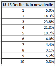
Let us break down that top decile.

This table shows what percent of top decile in the first period ended up in each decile of the second period. As we can see only 6% of the top decile runs in the first period ended up in the top decile in the second time period. Ouch! And .8% fell all the way to the bottom. The worst drop went from a rank of 159 to a rank of 2310. One piece of good news is that 77% of the runs stayed in the top 5 deciles.
Think about this numbers and if you do out of sample testing.
Spreadsheet
Fill the form below to get the spreadsheet with lots of more information. It contains all 2520 runs with yearly returns and decile information. A pivot table is included so you can do your analysis.
Final Thoughts
This is one reason when choosing a variation to trade from an optimization run that I do not like to pick anything near the top. I also set my expectations for future performance to be lower. In my next post, I will dive more into this topic. Post any comments on what you data you would like to see from this.
Backtesting platform used: AmiBroker. Data provider:Norgate Data (referral link)
Good Quant Trading

Fill in for free spreadsheet:
![]()

